Lecture 0: Introduction to Python#
Objective: #
My primary concern is to spark interest in a subject as challenging as computer programming. My approach isn’t heavily focused on pure algorithmics, but this is becoming less and less of a requirement for learning modern object-oriented programming. I also hope to open as many doors as possible with these notes. Indeed, it seems important to me to show that computer programming is a vast universe of concepts and methods, in which everyone can find their area of interest. I want each student to develop skills somewhat different from those of others, tailored to their inclinations, allowing them to value themselves in their own eyes as well as in those of their peers, and also to make a specific contribution when asked to collaborate on large-scale projects. Moreover, emphasis is placed on manipulating different types of data structures, as these are the backbone of any software development. The ultimate goal for each student will be to complete an original programming project of significant importance. There are a large number of programming languages, each with its own advantages and disadvantages. One must be chosen. For my own beginnings in studying programming, I used Python, which is a very modern language with growing popularity.
0. Introduction#
0.0. Why Python?#
The Python programming language is an excellent option for both beginners and those with more advanced knowledge. It is a high-level language with a syntax that encourages writing clear and high-quality code. Additionally, learning Python is facilitated by the existence of an interactive interface, particularly through the use of Jupyter notebooks. That said, its appeal goes beyond just learning programming or algorithms; its popularity and usage extend well beyond the academic realm, as evidenced by its growing popularity. It has been chosen by major players such as Google, YouTube, and NASA.
Python is a general-purpose programming language (i.e., serving multiple purposes and applicable to various fields of computer science). It is an interpreted language (meaning each line of code is read and then interpreted to be executed) rather than a compiled language. One of Python’s greatest strengths is its portability, meaning its ability to run on different platforms (Mac OS X, Unix, Windows, etc.). It operates with an object-oriented approach and provides a complete development environment that includes, in addition to an interpreter, a set of libraries. It has numerous modules that offer flexibility in their usage: writing web applications (Django), scientific calculations, data processing, text processing, data analysis, network management (socket library), access to relational databases, etc. This great flexibility and its ability to integrate into different technical environments make it a top choice for Big Data analysis.
The main features of the Python language:
Simple and readable syntax: educational language that is easy to learn and use;
Interpreted language: interactive use or line-by-line script execution, no compilation process;
High-level: dynamic typing, active memory management, for greater ease of use;
Multi-paradigm: imperative and/or object-oriented language, depending on individual needs and capabilities;
Free and open-source software, widely spread (multi-platform) and used (strong community);
Rich standard library: Batteries included;
Rich external library: many high-quality libraries available in various fields (including scientific).
Different versions of Python (for Windows, Unix, etc.), its original tutorial, its reference manual, the documentation for function libraries, etc., are available for free download from the official website.
The goal of this course is to learn a single high-level language, which allows for both quick analyses in everyday life – with just a few lines of interactive code – as well as more complex programs (larger projects, e.g., more than 100,000 lines).
0.1. Prerequisites#
This notebook introduces the free Python language and describes the initial commands necessary to get started with the language. The content is accessible to both beginners and relatively experienced users. It is well-suited for someone who wants to learn Python programming, but it also contains the essentials for getting acquainted with data analysis.
For more in-depth study, there are numerous educational resources available online. For example, the official tutorial for Python 3.4 provides abundant information for beginners. There is also Sheppard’s (2014) book, which offers an introduction to Python for Econometrics, Statistics, and Data Analysis, and Mac Kinney’s (2013) book, the principal author of the pandas library that we will discuss in a later notebook.
In addition to this introductory chapter on the basics of the Python language, you can also benefit from consulting the first five sections of the official tutorial for Python.
0.2. Installation#
Python and its libraries can be installed on almost any operating system from the official site. Here, we list the main scientific libraries useful for scientific computing and for defining essential data structures and calculation functions:
ipython: for interactive use of Python,numpy: for working with vectors and arrays,scipy: integrates key numerical algorithms,matplotlib: for plotting graphs,pandas: for data structures and spreadsheets,patsy: for statistical formulas,statsmodels: for statistical modeling,seaborn: for data visualization,scikit-learn: for statistical learning algorithms,sympy: for symbolic computation.
0.3. Python 2.7 vs. 3 (or more specifically, Python 2.7 vs 3.5)#
I will briefly discuss the differences between Python 2.x and Python 3.x. Although this is not a major issue for this course, I think it’s worth mentioning. Python comes in several versions that may be suitable for econometrics, statistics, and numerical analysis. Python 2.7 is the final version of the Python 2.x series — all future development work will focus on Python 3. Most differences between Python 2.7 and 3 are not critical for using Python in econometrics, statistics, and numerical analysis, i.e., scientific computing in general.
Here, I mention four notable differences that will allow you to use 2.7 and 3 interchangeably. Note that these differences are relatively significant in standalone Python programs.
print
print() is a function used to display text in the console when running programs. In Python 2.7, print is a keyword that behaves differently from other functions. In Python 3, print behaves like most other functions. The standard usage in Python 2.7 is
print "Strings to display."
whereas in Python 3, the standard usage is
print("Strings to display.")
which resembles the call of a standard function. Python 2.7 includes a version of the Python 3 print function, which can be used in any program by including:
from __future__ import print_function
at the top of the program.
division
Python 3 changes the way integers are divided. In Python 2.7, the division of two integers always resulted in an integer, and so the results were truncated toward 0 if the result was fractional. For example, in Python 2.7, 9/5 is 1. Python 3 gracefully converts the result to a floating-point number, so in Python 3, 9/5 is 1.8. When working with numerical data, automatic conversion of divisions helps avoid some rare errors. Python 2.7 can use Python 3’s behavior by including:
from __future__ import division
at the top of the program.
range andxrange
It is often useful to generate a sequence of numbers for iteration over some data. In Python 2.7, the best practice is to use the keyword xrange for this purpose, while in Python 3, this keyword has been renamed to range.
Unicode Strings
In Python 3, text strings are Unicode by default. In Python 2, strings are stored in ASCII by default—you need to add a “u” if you want to store Unicode strings in Python 2.x. This is important because Unicode is more versatile than ASCII. Unicode strings can store foreign language letters, Roman numerals, symbols, emojis, etc., giving you more options. In practice, this is unlikely to affect numeric code written in Python except possibly when reading or writing data. If you work in a language context where characters outside the standard 128-character ASCII set are used but are limited to those commonly encountered, it may be useful to use:
from __future__ import unicode_literals
to aid future compatibility when transitioning to Python 3.
You can read more about these differences and other technical details on the following pages:
1. Using Python#
Python executes programs or scripts. This language also runs interactively using a command interpreter (IDLE) or {IPython}. In educational settings, using and creating a Jupyter notebook (formerly IPython notebook) through a simple browser (avoiding Internet Explorer) is preferred.
Python Environments#
You can run Python in various ways, including creating scripts or using the Python interpreter. There are several integrated development environments (IDEs) available:
PyCharm: A popular Python IDE by JetBrains with a range of features including code analysis, a debugger, and an integrated development environment for web development.
Spyder: An open-source IDE specifically designed for scientific computing and data analysis in Python, providing features such as an interactive console and variable explorer.
PyDev for Eclipse: A Python IDE plugin for Eclipse, offering features such as code completion, debugging, and interactive console integration.
Rodeo: An IDE for data science and analytics, providing a user-friendly interface similar to RStudio, designed to handle Python code, data exploration, and visualization.
Sublime Text: A versatile text editor with support for Python development through various plugins and packages.
LiClipse: An Eclipse-based IDE that enhances the basic Eclipse features with additional support for Python and other languages.
Ninja IDE: A cross-platform IDE with support for Python development, offering features like a debugger, code completion, and project management.
Komodo IDE: A powerful IDE for multiple languages including Python, known for its advanced features such as debugging, code profiling, and version control integration.
You can also run Python using the Jupyter notebook. This allows you to save your commands, do more than simple development, and is the approach we will follow.
Jupyter Notebook#
Commands are grouped into cells followed by their results after execution. These results and comments are stored in a specific .ipynb file and saved. LaTeX commands are accepted for integrating formulas, and the layout is managed using HTML tags or Markdown.
The save command also allows you to extract only the Python commands into a .py file. This is a simple and effective way to keep a complete history of an analysis for presentations or creating tutorials. The notebook can be loaded in different formats: .html page, .pdf file, or slideshow. Additional extensions might need to be installed. You can find a list of available extensions here.
According to the Jupyter project, it provides this notebook environment for most programming languages (Python, Julia, …). It becomes an essential tool for ensuring the reproducibility of analyses.
Opening a notebook (IPython or Jupyter) in a browser can be done, depending on the installation, through menus or by executing:
jupyter notebook.
Some Guidelines for Effective Use of the Notebook#
Although learning to navigate a Jupyter notebook could be covered in a tutorial, users will find it intuitive as the tabs at the top of the page are self-explanatory. Tutorials can be read on the Jupyter project site. However, here are a few small pointers:
Once the notebook is open:
Enter Python commands in a cell.
Click the cell execution button (or use
Shift + EnterorCtrl + Enter):Shift + Enterexecutes the current cell and moves the cursor to the next cell.Ctrl + Enterexecutes the current cell and keeps the cursor in the same cell.
Add comment cells and HTML or Markdown tags.
Iterate by adding cells as needed. Once execution is complete:
Save the
.ipynbnotebook.Optionally, export to a
.htmlversion for a web page.Export the
.pyfile containing the Python commands for an operational version.
Executing Files#
It is possible to execute scripts (with the .py extension) from within a Jupyter notebook using the magic command %run. Note that the script you want to execute must be saved in the same directory as the current notebook.
%run hello.py
hello world
Are you looking for me?
                               ..  .  .           .
                                    :,.     ?NI  .
                    ..       .:::?MMMMMMMMMMMMMM8=..:~,   .  .
                        8MMMMMMMMMMMMMMMMMMMMMMMMMMMMMMMMMM?
                    .:$MMMMMMMMMMMMMMMMMMMMMMMMMMMMMMMMMMMMMM,
              . DMMMMMMMMMMMMMMMMMMMMMMMMMMMMMMMMMMMMMMMMMMMMMMM,.
              MMMMMMMMMMMMMMMMMMMMMMMMMMMMMMMMMMMMMMMMMMMMMMMMMMM
             MMMMMMMMMMMMMMMMMMMMMMMMMMMMMMMMMMMMMMMMMMMMMMMMMMMMMN~
         .  8MMMMMMMMMMMMMMMMMMMMMMMMMMMMMMMMMMMMMMMMMMMMMMMMMMMMMMMM,.
          $MMMMMMMMMMMMMMMMMMMMMMMMMMMMMMMMMMMMMMMMMMMMMMMMMMMMMMMMMMM
        .8MMMMMMMMMMMMMMMMMMMMMMMMMMMMMMMMMMMMMMMMMMMMMMMMMMMMMMMMMMMM, ..
        ZMMMMMMMMMMMMMMMMMMMMMMMMMMMMMMMMMMMMMMMMMMMMMMMMMMMMMMMMMMMMMM
        MMMMMMMMMMMMMMMMMMMMMMMMMMMMMMMMMMMMMMMMMMMMMMMMMMMMMMMMMMMMMMMM8
   .   NMMMMMMMMMMMMMMMMMMMMMMMMMMMMMMMMMMMMMMMMMMMMMMMMMMMMMMMMMMMMMMMMM=
    .?MMMMMMMMMMMMMMMMMMMMMMMMMMMMMMMMMMMMMMMMMMMMMMMMMMMMMMMMMMMMMMMMMMMZ
    =MMMMMMMMMMMMMMMMMMMMMMMMMMMMMMMMMMMMMMMMMMMMMMMMMMMMMMMMMMMMMMMMMMMMMM
    MMMMMMMMMMMMMMMMMMMMMMMMMMMMMMMMMMMMMMMMMMMMMMMMMMMMMMMMMMMMMMMMMMMMMMMM.
   .MMMMMMMMMMMMMMMMMMMMMMMMMMMMMMMMMMMMMMMMMMMMMMMMMMMMZ  +MMMMMMMMMMMMMMMMO
   .MMMMMMMMMMMMMMMMMMMMMMMMMMMMMMMMMMMMMMM .MM~.ZIMMMM .   ~MMMMMMMMMMMMMMM?
    NMMMMMMMMMMMMMMMMMIDD, =+MOMM,    8$M.~    .. .,MM8.     MMMMMMMMMMMMMMN
   8MMMMMMMMMMMMMMMM.                               .        8MMMMMMMMMMMMMN .
  .MMMMMMMMMMMMMMMMM,.       .                              .MMMMMMMMMMMMMMMO
  ,MMMMMMMMMMMMMMMMMO                                      ..MMMMMMMMMMMMMMM~
   DMMMMMMMMMMMMMMMMM                                       :MMMMMMMMMMMMMMM:
   IMMMMMMMMMMMMMMMMMO                                     . MMMMMMMMMMMMMMM+
   IMMMMMMMMMMMMMMMMM      .                       .       . +MMMMMMMMMMMMMM:
   :MMMMMMMMMMMMMMMMO                                        ,MMMMMMMMMMMMMM
   NMMMMMMMMMMMMMMMMD   ~NMMD.                    ..7OMMMMMO .MMMMMMMMMMMMM7
. .MMMMMMMMMMMMMMMMMM  NMNNMMMMMMN8         .   OMMMMM$.   ,O MMMMMMMMMMMM~  .
   MMMMMMMMMMMMMMMMM7 .         IMMMM.      . .7. . .=$7?   . .MM?MMMMMMM
    +MMMMMMMMMMMMMMM.    .ZMMMMMMM8, :  . .  D. Z$MMMMO.$MM    M$ MMMMMMM
    ..MMMMMMMMM:8 MM... . NM $M=M.O,N :, .  ,. 78: IMN I:N    .8 ~MMMMMMM8
   . ?MMMMMMMMMD. ZO.   .  ZI$I$O+~= ? O    =...::~$Z$8+       8 MMMMMMMMM
    .?MMMMMMMMMM  $$.       . ...      + .  ~.         .      .7 MMMMMMMM=
      MMMMMMMMMM= O~..              ..      ~.               ..7~MMMMMMMI
        DMMMMMMMM,M.O                       ,.             ...=.NMMMMMMMO
   .  .  MMMMMMMMM  M                       .~.               Z.MMMMMMMMM
         7MMMMMMMM8 M                        O                MMMMMMMMMM:.
         ?MMMMMMMMM8M              .         +                MMMMMMMMMM  .
        .MMMMMMMMMMMM              ~            .$         ..:MMMMMMMMM..
        ZMMMMMMMMMMMM:         .  ,.          .  ,=          +M ~OMMMM7~::::.
       .,MMMMMMMMMMMM7           .:I.7~      MMD?M         . 8~   .       .
         =MMMMMMMMMMMM             .DMO DD?D,+               M.           ..
          MMMMMMMMMMMM,           . ~MMMMMMMMMMMN:          ,8
       .   ,MMMMMMMMMMM           $MMMMMMMMMMMMMMMM8        M~
            OMMMMMMMMMM=        OMMMMMMMMMIMMMMMMMMMM7     =M
           .  ,MMMMMMM+.7      7MMMMI.     .  ..:=MMMM.  .$8.
                    M~  :Z     .ND88NND?,.  .?DN8O,$~I   :Z
                   D+ .  .M     .7,      ~87      M   ..~I
                  7I  .    M   .. .Z       ..    M    .+Z.
                 ,N         M    .  8.     . ..$~.    :$
            ..  .M.        . M.  .  . D+    =D:.     ,N
              $M~             M   .     .,.  .  .   .M
          . +D.               .~+                  .M
          .DO                   ,O              .  M
        ,M+                      .M.      ..     =M
    ..+M?..                        =M7.  .     ?M? .
   .D8   .                       .... .?8MMMNO?  .   .
  +.

                                                                 GlassGiant.com
Getting Help#
Finding your way around can be done with the help feature. To get help on the int type in Python, you can use the help() function. Here’s how you can do it in a Jupyter notebook or Python environment:
help(int)
This will display information about the int type, including its methods and how it can be used.
help(int)
Help on class int in module builtins:

class int(object)
 |  int([x]) -> integer
 |  int(x, base=10) -> integer
 |
 |  Convert a number or string to an integer, or return 0 if no arguments
 |  are given.  If x is a number, return x.__int__().  For floating point
 |  numbers, this truncates towards zero.
 |
 |  If x is not a number or if base is given, then x must be a string,
 |  bytes, or bytearray instance representing an integer literal in the
 |  given base.  The literal can be preceded by '+' or '-' and be surrounded
 |  by whitespace.  The base defaults to 10.  Valid bases are 0 and 2-36.
 |  Base 0 means to interpret the base from the string as an integer literal.
 |  >>> int('0b100', base=0)
 |  4
 |
 |  Built-in subclasses:
 |      bool
 |
 |  Methods defined here:
 |
 |  __abs__(self, /)
 |      abs(self)
 |
 |  __add__(self, value, /)
 |      Return self+value.
 |
 |  __and__(self, value, /)
 |      Return self&value.
 |
 |  __bool__(self, /)
 |      True if self else False
 |
 |  __ceil__(...)
 |      Ceiling of an Integral returns itself.
 |
 |  __divmod__(self, value, /)
 |      Return divmod(self, value).
 |
 |  __eq__(self, value, /)
 |      Return self==value.
 |
 |  __float__(self, /)
 |      float(self)
 |
 |  __floor__(...)
 |      Flooring an Integral returns itself.
 |
 |  __floordiv__(self, value, /)
 |      Return self//value.
 |
 |  __format__(self, format_spec, /)
 |      Default object formatter.
 |
 |  __ge__(self, value, /)
 |      Return self>=value.
 |
 |  __getattribute__(self, name, /)
 |      Return getattr(self, name).
 |
 |  __getnewargs__(self, /)
 |
 |  __gt__(self, value, /)
 |      Return self>value.
 |
 |  __hash__(self, /)
 |      Return hash(self).
 |
 |  __index__(self, /)
 |      Return self converted to an integer, if self is suitable for use as an index into a list.
 |
 |  __int__(self, /)
 |      int(self)
 |
 |  __invert__(self, /)
 |      ~self
 |
 |  __le__(self, value, /)
 |      Return self<=value.
 |
 |  __lshift__(self, value, /)
 |      Return self<<value.
 |
 |  __lt__(self, value, /)
 |      Return self<value.
 |
 |  __mod__(self, value, /)
 |      Return self%value.
 |
 |  __mul__(self, value, /)
 |      Return self*value.
 |
 |  __ne__(self, value, /)
 |      Return self!=value.
 |
 |  __neg__(self, /)
 |      -self
 |
 |  __or__(self, value, /)
 |      Return self|value.
 |
 |  __pos__(self, /)
 |      +self
 |
 |  __pow__(self, value, mod=None, /)
 |      Return pow(self, value, mod).
 |
 |  __radd__(self, value, /)
 |      Return value+self.
 |
 |  __rand__(self, value, /)
 |      Return value&self.
 |
 |  __rdivmod__(self, value, /)
 |      Return divmod(value, self).
 |
 |  __repr__(self, /)
 |      Return repr(self).
 |
 |  __rfloordiv__(self, value, /)
 |      Return value//self.
 |
 |  __rlshift__(self, value, /)
 |      Return value<<self.
 |
 |  __rmod__(self, value, /)
 |      Return value%self.
 |
 |  __rmul__(self, value, /)
 |      Return value*self.
 |
 |  __ror__(self, value, /)
 |      Return value|self.
 |
 |  __round__(...)
 |      Rounding an Integral returns itself.
 |
 |      Rounding with an ndigits argument also returns an integer.
 |
 |  __rpow__(self, value, mod=None, /)
 |      Return pow(value, self, mod).
 |
 |  __rrshift__(self, value, /)
 |      Return value>>self.
 |
 |  __rshift__(self, value, /)
 |      Return self>>value.
 |
 |  __rsub__(self, value, /)
 |      Return value-self.
 |
 |  __rtruediv__(self, value, /)
 |      Return value/self.
 |
 |  __rxor__(self, value, /)
 |      Return value^self.
 |
 |  __sizeof__(self, /)
 |      Returns size in memory, in bytes.
 |
 |  __sub__(self, value, /)
 |      Return self-value.
 |
 |  __truediv__(self, value, /)
 |      Return self/value.
 |
 |  __trunc__(...)
 |      Truncating an Integral returns itself.
 |
 |  __xor__(self, value, /)
 |      Return self^value.
 |
 |  as_integer_ratio(self, /)
 |      Return integer ratio.
 |
 |      Return a pair of integers, whose ratio is exactly equal to the original int
 |      and with a positive denominator.
 |
 |      >>> (10).as_integer_ratio()
 |      (10, 1)
 |      >>> (-10).as_integer_ratio()
 |      (-10, 1)
 |      >>> (0).as_integer_ratio()
 |      (0, 1)
 |
 |  bit_count(self, /)
 |      Number of ones in the binary representation of the absolute value of self.
 |
 |      Also known as the population count.
 |
 |      >>> bin(13)
 |      '0b1101'
 |      >>> (13).bit_count()
 |      3
 |
 |  bit_length(self, /)
 |      Number of bits necessary to represent self in binary.
 |
 |      >>> bin(37)
 |      '0b100101'
 |      >>> (37).bit_length()
 |      6
 |
 |  conjugate(...)
 |      Returns self, the complex conjugate of any int.
 |
 |  to_bytes(self, /, length=1, byteorder='big', *, signed=False)
 |      Return an array of bytes representing an integer.
 |
 |      length
 |        Length of bytes object to use.  An OverflowError is raised if the
 |        integer is not representable with the given number of bytes.  Default
 |        is length 1.
 |      byteorder
 |        The byte order used to represent the integer.  If byteorder is 'big',
 |        the most significant byte is at the beginning of the byte array.  If
 |        byteorder is 'little', the most significant byte is at the end of the
 |        byte array.  To request the native byte order of the host system, use
 |        `sys.byteorder' as the byte order value.  Default is to use 'big'.
 |      signed
 |        Determines whether two's complement is used to represent the integer.
 |        If signed is False and a negative integer is given, an OverflowError
 |        is raised.
 |
 |  ----------------------------------------------------------------------
 |  Class methods defined here:
 |
 |  from_bytes(bytes, byteorder='big', *, signed=False) from builtins.type
 |      Return the integer represented by the given array of bytes.
 |
 |      bytes
 |        Holds the array of bytes to convert.  The argument must either
 |        support the buffer protocol or be an iterable object producing bytes.
 |        Bytes and bytearray are examples of built-in objects that support the
 |        buffer protocol.
 |      byteorder
 |        The byte order used to represent the integer.  If byteorder is 'big',
 |        the most significant byte is at the beginning of the byte array.  If
 |        byteorder is 'little', the most significant byte is at the end of the
 |        byte array.  To request the native byte order of the host system, use
 |        `sys.byteorder' as the byte order value.  Default is to use 'big'.
 |      signed
 |        Indicates whether two's complement is used to represent the integer.
 |
 |  ----------------------------------------------------------------------
 |  Static methods defined here:
 |
 |  __new__(*args, **kwargs) from builtins.type
 |      Create and return a new object.  See help(type) for accurate signature.
 |
 |  ----------------------------------------------------------------------
 |  Data descriptors defined here:
 |
 |  denominator
 |      the denominator of a rational number in lowest terms
 |
 |  imag
 |      the imaginary part of a complex number
 |
 |  numerator
 |      the numerator of a rational number in lowest terms
 |
 |  real
 |      the real part of a complex number
In a Jupyter notebook, you can use the ? syntax to get a simplified version of the help for the int type:
int?
This will display a brief overview of the int type, including a summary of its methods and usage.
int?
Resetting Jupyter#
The magic command %reset is used to reset the notebook. It clears all variables existing in the current session.
To use it, simply type:
%reset
This command will prompt you to confirm the reset. If you want to reset without confirmation, you can use:
%reset -f
my_char1 = "Let's do the necessary."
print(my_char1)
Let's do the necessary.
%reset
Once deleted, variables cannot be recovered. Proceed (y/[n])? y
print(my_char1)
---------------------------------------------------------------------------
NameError                                 Traceback (most recent call last)
Cell In [6], line 1
----> 1 print(my_char1)

NameError: name 'my_char1' is not defined
my_char2 = "Have we done it?"
print(my_char2)
Have we done it?
%reset -f
print(my_char2)
---------------------------------------------------------------------------
NameError                                 Traceback (most recent call last)
Cell In [9], line 1
----> 1 print(my_char2)

NameError: name 'my_char2' is not defined
2. Date types#
2.0 Scalars and Strings#
Variable declaration is implicit (e.g., integer, float, boolean, string).
a = 4  # is an integer
b = 2.  # is a float

# Note:
a/2  # the result is 1.5 in Python 3.4
     # but 1 in 2.7
2.0
Comparison operators: ==, >, <, != return a boolean result. They return True or False.
In Python, a == b is a comparison operator used to check if the value of a is equal to the value of b. It returns True if a and b are equal, and False otherwise.
For example:
a = 5
b = 10
print(a == b)  # This will print False because 5 is not equal to 10
# Comparaison
a == b
False
In Python, type(a) is used to determine the type of the variable a. It returns the type of a as a type object.
For example:
a = 5
print(type(a))  # This will print <class 'int'> because 'a' is an integer

b = 3.14
print(type(b))  # This will print <class 'float'> because 'b' is a float

c = "Hello"
print(type(c))  # This will print <class 'str'> because 'c' is a string
If you have any specific questions about variable types or need more examples, let me know!
type(a)
int
In Python, concatenating strings is straightforward using the + operator. When you add strings together, they are combined into a single string.
Here is the example you provided:
a = 'bonjour '
b = 'tout le '
c = 'monde'
d = 'la famille'

result = a + b + c
print(result)  # This will print 'bonjour tout le monde'
In this case, a + b + c combines the strings 'bonjour ', 'tout le ', and 'monde' into the single string 'bonjour tout le monde'.
# Chaîne de caractère
a = 'bonjour '
b = 'tout le '
c = 'monde'
d = 'la famille'
a + b + c
'bonjour tout le monde'
a + d
'bonjour la famille'
2.1 Basic Structures#
Lists#
Lists allow combinations of types. Note: The first element of a list or array is indexed by 0, not by 1.
Initializing Lists#
liste_A = [1, 34, 52, 'Slt']
liste_B = [0, 3, 209, 4025, 554, 6, 1]
liste_C = [0, 53, 562, 'rdv', [17, "l", 298, 43]]
### Initializing Lists
liste_A = [1, 34, 52, 'Slt']
liste_B = [0, 3, 209, 4025, 554, 6, 1]
liste_C = [0, 53, 562, 'rdv', [17, "l", 298, 43]]
In Python, to access an element in a list, you use indexing. Here’s how you access an element from liste_A:
# Accessing an element from the list
liste_A[1]
This will return 34, as indexing starts from 0, so liste_A[1] refers to the second element in the list.
# Entry of a list
liste_A[1]
34
liste_C[-1] # last entry
[17, 'l', 298, 43]
liste_C[3] = 45 # Modify an entry of the list
liste_C
[0, 53, 562, 45, [17, 'l', 298, 43]]
To access elements within a nested list, you use multiple indices. In this case, list_C[-1] refers to the last element of list_C, which is itself a list. To access elements within this nested list, you use an additional index.
For example:
# Accessing the first element of the last list in list_C
liste_C[-1][0]
This will return 17, as list_C[-1] refers to [17, "l", 298, 43], and [0] accesses the first element of this nested list.
liste_C[-1][0]
17
The expression liste_B[0:2] is used to create a sublist from liste_B, including elements from index 0 up to but not including index 2. In Python, slicing is performed using the format list[start:end], where start is the index to begin the slice (inclusive) and end is the index to end the slice (exclusive).
For example:
# Given list_B
liste_B = [0, 3, 209, 4025, 554, 6, 1]

# Creating a sublist from index 0 to 2 (not including 2)
sous_liste = liste_B[0:2]
print(sous_liste)  # Output: [0, 3]
Here, sous_liste will contain the elements [0, 3], which are the elements at indices 0 and 1 of liste_B.
liste_B[0:2] # Sublist, runs throuh liste_B at the indices 0 and 1.
[0, 3]
The expression liste_B[0:5:2] is used for slicing with a step. It extracts elements from liste_B starting at index 0, up to but not including index 5, with a step of 2.
In this case:
0is the starting index (inclusive).5is the ending index (exclusive).2is the step, meaning every second element is selected.
Here’s how it works:
# Given list_B
liste_B = [0, 3, 209, 4025, 554, 6, 1]

# Slicing with start=0, end=5, and step=2
sous_liste = liste_B[0:5:2]
print(sous_liste)  # Output: [0, 209, 554]
In this example, sous_liste contains [0, 209, 554], which are the elements at indices 0, 2, and 4 of liste_B.
liste_B[0:5:2] # start:end:step
[0, 209, 554]
What is happening here ?#
liste_B[::-1]# Comprendre ce qui se passe ici
[1, 6, 554, 4025, 209, 3, 0]
The expression liste_B[::-1] is used for reversing a list.
Here’s a breakdown of how it works:
:specifies that the slicing should include the entire list.The first
:indicates the start and end of the slice, but since both are omitted, it defaults to the entire list.The
-1is the step, which tells Python to take elements in reverse order.
So, liste_B[::-1] creates a reversed copy of liste_B.
Here’s an example:
# Given list_B
liste_B = [0, 3, 209, 4025, 554, 6, 1]

# Reversing the list
reversed_list = liste_B[::-1]
print(reversed_list)  # Output: [1, 6, 554, 4025, 209, 3, 0]
In this example, reversed_list is the reverse of liste_B, with the elements in the opposite order.
# Methods on lists
List = [333,276,4827,187,984]
List.sort()
print(List)
[187, 276, 333, 984, 4827]
List.append('hi') # Add an entry an the end
print(List)
[187, 276, 333, 984, 4827, 'hi']
List.count(3) # "Counts the number of times the entry '3' appears"
0
Observe the difference between the two methods .append() and .extend().#
List.extend([7,8,9])
print(List)
[187, 276, 333, 984, 4827, 'hi', 7, 8, 9]
List.append([10,11,12])
print(List)
[187, 276, 333, 984, 4827, 'hi', 7, 8, 9, [10, 11, 12]]
Tuple#
A tuple is similar to a list but cannot be modified; it is defined by parentheses.
MyTuple = (2020,34,42,'h')
MyTuple[1]
34
MyTuple[1] = 10 # TypeError: "tuple" object
# You cannot modify an entry in a tuple, unlike lists
---------------------------------------------------------------------------
TypeError                                 Traceback (most recent call last)
Cell In [29], line 1
----> 1 MyTuple[1] = 10 # TypeError: "tuple" object
      2 # You cannot modify an entry in a tuple, unlike lists

TypeError: 'tuple' object does not support item assignment
Dictionary#
A dictionary is similar to a list, but each entry is assigned by a key/name and is defined with curly braces. This object is used for constructing column indexes (variables) of the DataFrame type in the pandas library.
months = {'Jan':31 , 'Fev': 29, 'Mar':31, 'Apr':30}
mois['Apr']
---------------------------------------------------------------------------
NameError                                 Traceback (most recent call last)
Cell In [30], line 2
      1 months = {'Jan':31 , 'Fev': 29, 'Mar':31, 'Apr':30}
----> 2 mois['Apr']

NameError: name 'mois' is not defined
The methods .values(), .keys(), and .items() are very useful for a dictionary.
months.values()
dict_values([31, 29, 31, 30])
months.keys()
dict_keys(['Jan', 'Fev', 'Mar', 'Apr'])
months.items()
dict_items([('Jan', 31), ('Fev', 29), ('Mar', 31), ('Apr', 30)])
Create a dataframe with pandas#
To create a DataFrame with pandas, you can follow these steps:
Import pandas: First, ensure that you have pandas installed and import it into your Python environment.
import pandas as pd
Create a DataFrame: You can create a DataFrame using various methods such as from a dictionary, list of lists, or other data structures.
From a dictionary:
data = {
    'Column1': [1, 2, 3],
    'Column2': ['A', 'B', 'C']
}
df = pd.DataFrame(data)
From a list of lists:
data = [
    [1, 'A'],
    [2, 'B'],
    [3, 'C']
]
df = pd.DataFrame(data, columns=['Column1', 'Column2'])
From a CSV file:
df = pd.read_csv('path_to_file.csv')
Inspect the DataFrame: Use methods to view the DataFrame and understand its structure.
print(df.head())  # View the first few rows
print(df.info())  # Get a summary of the DataFrame
print(df.describe())  # Get statistical summaries of numerical columns
Manipulate the DataFrame: Perform operations such as filtering, sorting, and aggregating.
# Filtering rows
filtered_df = df[df['Column1'] > 1]

# Sorting by a column
sorted_df = df.sort_values(by='Column1')

# Adding a new column
df['NewColumn'] = df['Column1'] * 10
This basic overview should help you get started with creating and manipulating DataFrames in pandas.
import pandas as pd  # Importing the pandas library with the alias "pd"
# Using lists and dictionaries.
# Gender and the number of hours spent in front of the TV.
# m = male; f = female
data = pd.DataFrame({
    'Gender': ['f', 'f', 'm', 'f', 'm', 'm', 'f', 'm', 'f', 'f'],
    'TV': [3.4, 3.5, 2.6, 4.7, 4.1, 4.0, 5.1, 4.0, 3.7, 2.1]})
data
| Gender | TV | |
|---|---|---|
| 0 | f | 3.4 |
| 1 | f | 3.5 |
| 2 | m | 2.6 |
| 3 | f | 4.7 |
| 4 | m | 4.1 |
| 5 | m | 4.0 |
| 6 | f | 5.1 |
| 7 | m | 4.0 |
| 8 | f | 3.7 |
| 9 | f | 2.1 |
3. Python Syntax#
Here’s an overview of basic Python syntax:
3.1 Variables and Data Types#
Variables: Store values. Python uses dynamic typing, so you don’t need to declare the type of a variable explicitly.
Data Types: Includes integers (
int), floating-point numbers (float), booleans (bool), and strings (str).
3.2 Operators#
Arithmetic Operators:
+,-,*,/,//(integer division),%(modulo),**(exponentiation)Comparison Operators:
==,!=,>,<,>=,<=Logical Operators:
and,or,not
3.3 Control Flow#
Conditional Statements: Use
if,elif, andelseto control the flow of your program based on conditions.if condition: # code block elif another_condition: # code block else: # code block
Loops:
For Loops: Iterate over a sequence (like a list or range).
for item in sequence:
    # code block
While Loops: Continue executing as long as a condition is true.
while condition:
    # code block
3.4 Functions#
Defining Functions: Use
defto define a function.def function_name(parameters): # code block return result
Calling Functions: Use the function name followed by parentheses.
result = function_name(arguments)
3.5 Lists and Dictionaries#
Lists: Ordered, mutable collections.
my_list = [1, 2, 3, 'a', 'b']
Dictionaries: Unordered collections of key-value pairs.
my_dict = {'key1': 'value1', 'key2': 'value2'}
3.6 Exception Handling#
Try-Except Blocks: Handle errors gracefully using
tryandexcept.try: # code block that might raise an exception except ExceptionType as e: # code block to handle the exception
3.8 Indentation#
Indentation: Python uses indentation to define code blocks. Consistent indentation is crucial for defining scope in control flow statements and function definitions.
Conditional Structure#
# **If-Then-Else**
a = -23
if a > 0:
    b = 0
    print(b)
else:
    b = -1
print(b)
-1
Iterative Structure#
for i in range(4):
    print(i)
0
1
2
3
for i in range(1,8,2):
    print(i)
1
3
5
7
Functions#
# Definition of a function
def pythagorus(x,y):
    """ "Calculate the hypotenuse of a triangle" """
    r = pow(x**2+y**2,0.5)
    return x,y,r
pythagorus(5,6)
(5, 6, 7.810249675906654)
# Example of a call
pythagorus(x=5,y=7)
(5, 7, 8.602325267042627)
# integrated help
help(pythagorus)
Help on function pythagorus in module __main__:

pythagorus(x, y)
    "Calculate the hypotenuse of a triangle"
pythagorus.__doc__
' "Calculate the hypotenuse of a triangle" '
Modules#
“A module contains several functions and commands grouped in a file with the .py extension. It is called using the import command.”
Start by defining a module in a text file with the following commands:
def DitBonjour():
    print("Bonjour")
def DivPar2(x):
    return x/2
Save the file as testM.py in the current directory.
It is possible to import all functions with a single import command.
import testM # import the module
testM.DitBonjour()
Bonjour
testM.DivPar2(7)
3.5
print(testM.DivPar2(10))
5.0
# We can also do
from testM import *
DitBonjour()
Bonjour
print(DivPar2(10))
5.0
# Or
import testM as tm
tm.DitBonjour()
Bonjour
print(tm.DivPar2(10))
# deletion of objects
5.0
# deletion of objects
%reset
Once deleted, variables cannot be recovered. Proceed (y/[n])? y
from testM import DitBonjour
## Only one function has been called. Prefer this method for large libraries.
DitBonjour()
Bonjour
print(DivPar2(10)) # error
---------------------------------------------------------------------------
NameError                                 Traceback (most recent call last)
Cell In [53], line 1
----> 1 print(DivPar2(10)) # error

NameError: name 'DivPar2' is not defined
4. Scientific Computing#
Here are three of the main libraries essential for scientific computing. Two other libraries: pandas and scikit-learn, are covered in detail in specific notebooks.
4.0 Packages#
NumPy#
This library defines the array data type and the associated computation functions. It also includes some linear algebra and statistical functions. However, numerical functions are much more extensive in SciPy.
SciPy#
This library is a very comprehensive collection of modules for linear algebra, statistics, and other numerical algorithms. The documentation site provides a complete list.
Matplotlib#
This library offers visualization/graph functions with commands similar to those in Matlab. It is also known as pylab. The gallery of this library features a wide range of example plots with Python code to generate them.
# Import
import numpy as np
from pylab import *
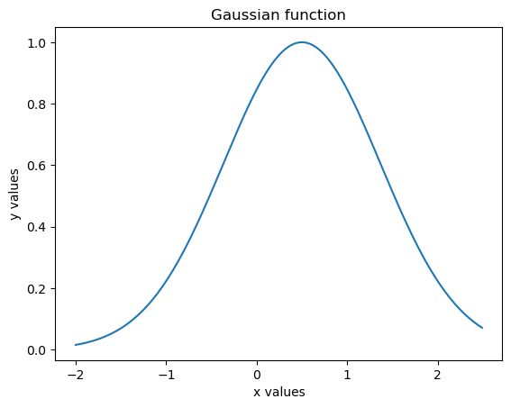
gaussian = lambda x: np.exp(-(0.5-x)**2/1.5)
x=np.arange(-2,2.5,0.01)
y=gaussian(x)
plot(x,y)
xlabel("x values")
ylabel("y values")
title("Gaussian function")
show()
4.1 Array Type#
This is by far the most commonly used data structure for scientific computing in Python. It describes arrays or multi-index matrices of dimension ( n = 1, 2, 3, \ldots, 40 ). All elements are of the same type (boolean, integer, real, complex).
Data tables (data frames), which are the basis for statistical analysis and aggregate objects of different types, are described using the pandas library.
Definition of the array Type#
# Import
import numpy as np
mon_tableau_en_dim1 = np.array([44,33,22])
print(mon_tableau_en_dim1 )
[44 33 22]
mon_tableau_in_dim2 = np.array([[1,0,0],[0,2,0],[0,0,3]]) # lignes & colones
print(mon_tableau_in_dim2)
[[1 0 0]
 [0 2 0]
 [0 0 3]]
MaListe = [121,245,398,872]
mon_tableau = np.array(MaListe)
print(mon_tableau)
[121 245 398 872]
a = np.array([[0,1],[2,3],[4,5]])
a[2,1]
5
a[:,1]
array([1, 3, 5])
type(a[:,1])
numpy.ndarray
Methods of type array#
np.arange(21)
array([ 0,  1,  2,  3,  4,  5,  6,  7,  8,  9, 10, 11, 12, 13, 14, 15, 16,
       17, 18, 19, 20])
np.ones(5)
array([1., 1., 1., 1., 1.])
np.ones((7,5))
array([[1., 1., 1., 1., 1.],
       [1., 1., 1., 1., 1.],
       [1., 1., 1., 1., 1.],
       [1., 1., 1., 1., 1.],
       [1., 1., 1., 1., 1.],
       [1., 1., 1., 1., 1.],
       [1., 1., 1., 1., 1.]])
np.eye(4)
array([[1., 0., 0., 0.],
       [0., 1., 0., 0.],
       [0., 0., 1., 0.],
       [0., 0., 0., 1.]])
np.linspace(3, 7, 3)
array([3., 5., 7.])
np.mgrid[0:3,0:2]
array([[[0, 0],
        [1, 1],
        [2, 2]],

       [[0, 1],
        [0, 1],
        [0, 1]]])
D = np.diag([111,202,904])
print(D)
print(np.diag(D))
[[111   0   0]
 [  0 202   0]
 [  0   0 904]]
[111 202 904]
M = np.array([[10*n+m for n in range(3)]
for m in range(2)])
print(M)
[[ 0 10 20]
 [ 1 11 21]]
The numpy.random module provides a whole range of functions for generating random matrices.
from numpy import random
random.rand(7,3) # uniform sampling
array([[0.53073701, 0.31297603, 0.5641477 ],
       [0.43777429, 0.83163615, 0.66496753],
       [0.24002488, 0.95816308, 0.57628792],
       [0.24424045, 0.89968047, 0.75104168],
       [0.1641301 , 0.44323146, 0.56220595],
       [0.4760593 , 0.01161395, 0.19141526],
       [0.51026382, 0.81099477, 0.48375166]])
random.randn(8,5) # **Sampling from the N(0,1) Distribution**
array([[ 0.88907886,  0.12507027,  0.09150879, -2.42828769, -0.2430704 ],
       [-1.83810087, -0.7139083 , -0.70324809,  1.03869728, -2.06852043],
       [ 0.54693172,  0.47675494,  1.13256001,  1.18915764,  0.82072297],
       [-1.08843424,  1.81255327, -2.29072737, -0.50313616,  0.30826458],
       [-0.97381724, -0.41838826,  0.85145296, -0.33294871, -0.18852696],
       [-1.4338638 , -0.16385629, -0.91086764,  0.4628748 , -0.45713318],
       [ 1.82422127,  0.62571939, -0.31407905,  0.00758607,  0.42176071],
       [ 0.97845495, -1.80729864, -0.18570848,  1.05945622,  0.12493888]])
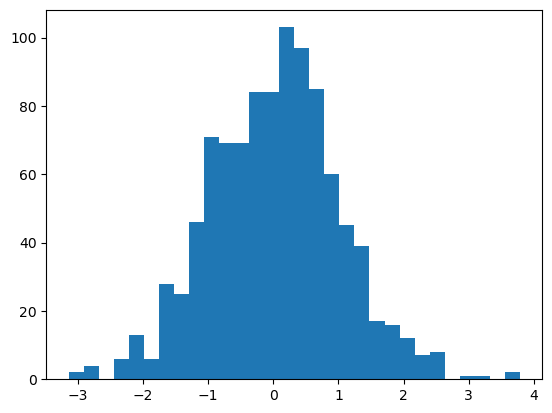
v = random.randn(1000)
import matplotlib.pyplot as plt
h = plt.hist(v,30) # **histogram with 30 Bins**
show()
Other functions#
a = np.array([[0,1],[2,3],[4,5]])
np.ndim(a) # Number of dimensions)
2
There are many functions you can test, including:
np.size(a)for the number of elements,np.shape(a)which returns a tuple containing the dimensions ofa,np.transpose(a)ora.Tfor the transpose,a.min()ornp.min(a)for the minimum value,a.sum()ornp.sum(a)for the sum of the values.
and many other functions.
Operations on arrays#
# Sum
a = np.arange(6).reshape(3,2)
b = np.arange(3,9).reshape(3,2)
c = np.transpose(b)
a + b
array([[ 3,  5],
       [ 7,  9],
       [11, 13]])
a * b # term-by-term product (element-wise product)
array([[ 0,  4],
       [10, 18],
       [28, 40]])
np.dot(a,c) # matrix product (or dot product)
array([[ 4,  6,  8],
       [18, 28, 38],
       [32, 50, 68]])
np.power(a,2)
array([[ 0,  1],
       [ 4,  9],
       [16, 25]])
In other notebooks that are fully developed on this topic, we will discuss the NumPy and SciPy libraries in more detail (should time permit). We conclude this introductory notebook with what we call programming structures, which form the backbone of this course.
Programming Structures#
Blocks are defined by indentation (usually by 4 spaces);
One statement per line generally (or statements separated by
;);Comments start with
#and extend to the end of the line;Boolean Expression: a condition is an expression that evaluates to
TrueorFalse:False: false logical test (e.g., 3 == 4), null value, empty string (‘’), empty list ([]), etc.,True: true logical test (e.g., 2 + 2 == 4), any non-null value or object (and thus evaluating to True by default except exceptions);Logical Tests:
==,!=,>,>=, etc.;Logical Operators:
and,or,not;Ternary Operator:
value **if** condition **else** value;
Conditional Expression:
**if** condition1 : ... [**elif** condition2 : ...] [**else**: ...];For Loop:
**for** element **in** iterable, executes on each element of an iterable object:continue: interrupts the current iteration and resumes the loop at the next iteration,break: completely interrupts the loop;
While Loop:
while condition: repeats as long as the condition is true, or after an explicit exit withbreak.
These structures will be discussed in detail in upcoming notebooks.
3.7 Comments#
Single-line Comments: Use
#to write comments.# This is a commentMulti-line Comments: Use triple quotes
'''or""".